Visitors since March 2003. Page update v8.73

note ** the navigation bars are currently not working correctly. When working in events, please select page 2 from the blank boxes at the top, the back and next bar will then move you throughout the event.

Please visit www.highgatehouse.co.uk  to see our range of  Vehicle, Circuit & Track decals and a lot more !

NEW! We now have available Coffee Mugs printed with your car pictures from our events pages. See SHOP for Details!

Torque, Power, and Kinematics

The following discussion of basic physical principles involved in kinematics and dynamics of automobiles may bore some of you. It may also enlighten you. The discussion will be in no way satisfactory for those that study such physical phenomena on professional level or are true enthusiasts seeking advanced understanding. Rather it will be light and informative by just slightly touching the mathematics and physics involved.  However, after reading the text and looking at the diagrams I hope that you will walk away with just a bit more understanding of the concept of power and torque.

In the consumer world of car salespeople, car magazines, internet groups dedicated to the wonder on four wheels, the words power and torque are heard a lot and used a lot. Ironically, very few people, according to my observation, know the precise definition and application of each terms as related to cars. What is better to have – more power or more torque? Are they related? Such questions puzzle many, but only few stray from pseudo-scientific explanations and myths. I will not try to answer these questions directly; rather I will give definitions and relations, letting  you find the answers for yourself.

Let us begin:

In our universe we’re given three independent quantities: length, time, and mass. All other quantities are derived from the three main ones.
Let us label them as:
 

L – length
T – time
M – mass

Then speed, for example, is s = L/T. Force is f = (M *L) / (T * T). Note that these quantities are independent from our system of measurement. Speed can be measured in Miles per Hour or Parsecs per Millennium.
 

Let us now define what torque and power are as a function of the three fundamental quantities:

Power is the rate at which one does work or  work per time.
Work is a force applied over a distance or force times distance.
Thus power is: p = (M * L * L) / (T * T * T).

Torque is force applied at a moment arm of a given length.

Thus torque is: t =  (M * L * L) / (T * T ).

Comparing the above two formulas, one can clearly see that the only difference between the two is that power has one more time factor in the denominator. One is wise to notice this because if there is a quantity that has a formula 1 / T and that is physically relevant, we can multiply it by torque to get power.
Such quantity does exist and in our case, due to the geometry of  force application, it is the rotational speed of the engine’s crankshaft or more simply, the engine speed.
Thus in our case:

Power = C *torque * engine speed.

What is that C doing there? That C is a factor that has to do with the measurement system that we’re using. If you happen to measure torque in ft-lb, engine speed in revolutions per minute (RPM), and  power in SAE horsepower, C comes out to about 1/5250.  If you happen to measure torque in meter-newtons, engine speed in radians per second, and power in Watts, C = 1.

Let us stick to our SAE motorheads measurement table. Then we have a formula relating torque and power:

Power = Torque * RPM / 5250

Great. Assuming it’s right, so what?

Well, consider we want to accelerate a car with mass m from 0 to speed s using an engine with constant power p. How much time will it take?
Well, the car will undergo an kinetic energy change of: k = (0.5 * m * s*s) – 0, or the difference between the kinetic energy of the car at rest and at  speed s.
Now this kinetic energy change was brought about by work done by the engine. Since we know that power is work per time, we know that by dividing total work done by the applied power, produces the time needed to do the work and thus time to accelerate the car.
So what does this  tell us? This tells us that it is the power that accelerates the car.

But what about torque?

Remember that:

Power = Torque * RPM / 5250.

Examine the formula carefully….
It says that power has two variable components – torque and engine speed. Naturally, the torque here is the "twisting force" developed at a particular engine speed. So there is more than just torque involved into accelerating the car. After all, you can apply torque all you want, but if the engine is not  spinning, there is no work done, no power produced and you're not moving anywhere.
Another interesting feature is that at 5250 RPM the numeric magnitudes of torque and power figure will always match in our measurement system,  irrespective of the number of cylinders, volume, valve train or any other such feature of  the engine. Cool, huh? This is a very fundamental notion because it tells us that power ALWAYS grows faster with increase in RPMs than torque does. We’ll see how that is used in engine building later.

Now that we’re armed  with this new understanding, let us examine a few idealized examples.
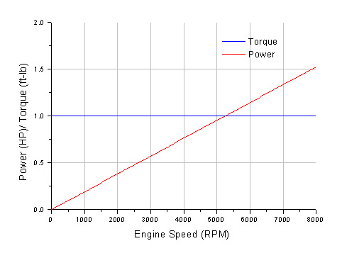
Consider an engine which develops exactly same torque T throughout its allowed RPM range. In this case torque is constant and:

Power = RPM * T/5250 which is a straight line with a slope T/5250 (see graph below).
How does this car  behave? Smooth and predictable. The power increases linearly and the higher RPMs you attain, the more power you develop all the way up to the redline. This is the ideal curve for an  engine – maximum torque everywhere in the range leaves only the RPM as the limiting factor. See graph below.
 
 

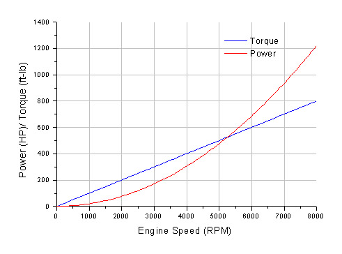
The next example is where torque is a linear function of the RPM.

Torque = a * RPM + b where a is the slope and b is the base torque developed when the engine is barely  moving.
From our trusty power/torque formula we deduce that in this case:

Power = (a * RPM * RPM + b *RPM) / 5250.

Not hard to see that power is a quadratic function of the RPM. Notice that power rises much faster,  as a square of RPM, than in the first example. Thus high power and acceleration can be attained, but you need to spin the engine faster. Notice that power is always rising faster than torque. See graph below.
 

So, what is important? Well, as you can see, at low RPM, if you want to develop lots of power, then you simply  need lots of torque at those engine speeds. That is why you hear – high low-end  torque being a good thing. But, in order to develop high low-end torque you either need a large engine or forced induction scheme. So the makers of small engines have focused their attention on the other side of the spectrum – high RPM side taking the advantage of the fundamental law that allows power to outgrow torque provided torque doesn't diminish too fast with rise in engine speed.   There, it’s the high RPMs that make horsepower even if the torque being developed is only marginal.

Tuning Engines, Valve Timing, and Smart Marketing

Now that we’re armed with understanding  of concept of torque and power, let’s see how we can develop  a simple model to gain an intuitive understanding of engine design and tuning.

Simplify the Problem

Let us consider an idealized internal combustion engine. We will assume that both intake and exhaust systems pose a constant restriction to flow regardless of engine speed. Our engine has a fixed volume, and fixed maximum compression.  These are usually fixed by space, fuel economy, and gasoline quality. We will come back to these later. No forced induction of any sort is used.

One of the most crucial aspects of engine tuning is valve timing. Whether fixed or variable, valve timing is a great compromise that engineers have to make when designing an engine.

Why is valve timing important?

While the octane ratio of gasoline, compression ratio, temperature of the engine, and engine volume determine the what force can be applied to the piston assuming you had a very long time to do it, and the cylinder was perfectly sealed (and what torque can be applied to the crank shaft),  the  valve timing controls just how much gas/air mixture gets into the cylinder, how much exhaust leaves the cylinder, and how well the combustion chamber is sealed during the compression and ignition.  An ideal case would be that the intake valves open, the air/fuel mixture comes to the point where the pressure inside the cylinder is equal to the pressure outside the engine, then the valves close and remain perfectly closed during compression and ignition and expansion. The exhaust valves instantly open and let all the exhaust gasses out of the combustion chamber and then the cycle repeats. This, however, is far from the way it occurs because of many limitations and engineering compromises.
 

One such compromise arises from the way that valves are actuated on modern cars. Currently, the only system on the market does the actuating by a shaft with cams on it (camshaft). Some engines have the shaft located high in the engine head itself (OHC) and some have it located low in the block. As the shaft rotates, so do the lobes (cams) attached to the shaft. When the lobe is in the right position, it presses either a rod, or a lifter which is connected to the valve. As it passes by, the lifter is pushed back by a spring and the valve closes again.

The main limitation of such design is the fact that the height of the cam , the width and when it pushes on the valve in relation to the piston position is constant regardless of engine speed. On the graph below, I have plotted what a torque profile of a cam might look like.

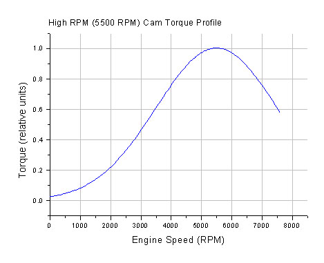
This is not a typical real cam profile (although in principle, it can be), as the torque is a gaussian function, but it will help us learn many interesting things about how valve timing affects the engine power and car drivability and performance. Gaussian function is a good choice because it has a certain width and certain height.

Physically, height is determined by the compression ratio, octane rating of gas, and other such things. This is the maximum torque than engine can produce using this cam. But does this profile correspond to how the car will accelerate? No! Remember – power is what accelerates the car which the product of the both the torque and engine speed!

But why does the torque fall of at lower RPM? This is because during low engine speed, valves stay open longer and compression leaks through open valves. Why does it fall of during very high RPM? Because there, the valves don’t open long and high enough to allow all gasses to enter or exit. Thus, any cam has a sweet spot.

Let us compute the power and plot it together woith torque. The units of power are relative and are not important in absolute sense. The graph below shows both torque and power developed by the camshaft. In this example, power outgrows torque numerically in our system if measurement.

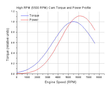
Notice a few important points here:

1. Torque peak occurs at 5500 RPM
2. Power peak is, however, at 6200 RPM

Let us now take a similar cam, but tune the valve timing to produce maximum torque at 3000 RPM. We’ll keep the profile of the cam the same and thus we’ll have the same height and width of the torque curve. Additionally, we’ll plot the high RPM cam and low RPM cam torque can  power curves on the same graphs for comparison.
 
 

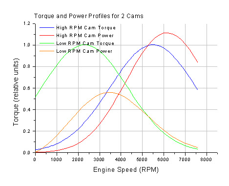
What can we see?

Well, we see that the lower rpm cam setup produces more power from 0 to almost 4300 RPM. This obviously means that at regular street driving, this engine will feel stronger and pull the car harder. How often does one go beyond 4000 RPM while driving in regular traffic?

However, after 4300 RPM, the high RPM cam takes off  and keeps making horsepower up to 6200 RPM when it finally falls off.
Remember that we’re just modifying the kinetics of gas flow in and out of the engine, nothing else. The effect is rather significant, don’t you think? So which one do you choose?

Well, for a good commuter car, I’d choose the low RPM cam as it provides a good low RPM power and has a nice broad power band. For a sports car though, I’d choose the high RPM cam, because it really shines and allows the engine to develop high horsepower at high engine speeds. So is there anything else missing from the formula?
Of course – gearing!  The gear ratios must be carefully chosen such that the engine speed is allowed to stay near the sweet spot of the power band at any car speed.

Perfecting the Solution

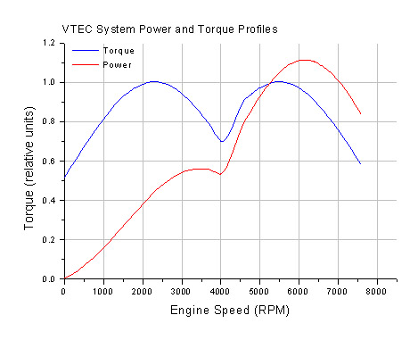
Engineers see the above, as one of the main foes of a “perfect” engine. So the latest trend is variable valve timing. The simplest, and one of the best, is the Honda’s VTEC system. This system can vary all three of the main valve timing parameters – phase, lift distance, and lift duration. Essentially, it allows switching between two different sets of cam lobes on the fly. The characteristics of each set of lobes can be chosen, for most part, independent of the other. So, in our model, we can combine the torque and power curves of the high and low RPM cams. (see Graph below) In effect, we switch from low RPM cam to high RPM cam at about 4300 RPM. Thus, we have the low end power of the low RPM cam and high RPM power of high RPM cam. Cool, huh?! See graph below.

There are other systems such Toyota’s VVTi which can continuously vary the phase of the cam lobes. In this case, imagine having a cam that can adjust such that you’re always close to the horsepower peak! It’s not quite that simple because of other limitations, but that’s the idea.

Another Solution

On the other side, we have CVTs - continuously variable transmissions. Using novel technologies, these can vary the gear ratio such that the engine always runs at the same speed regardless of the speed of the car. In that case, design of the cam will be very simple. Since power can be freely adjusted, you don’t need a wide power band.

As you see, there is more than one solution to these complex problems. And that is what makes engineering so interesting.
 

No Replacement for Displacement?

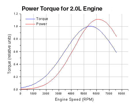
But let us get back to displacement and compression. Once again, these are the parameters that affect torque and thus affect power and acceleration. Let us start with a certain engine – say 2.0L. If we want to advertise high HP figures and sell this car in “sports” category, you now know what to do – design the cam and engine with a sweet spot at high RPM. Very good. So we peak our 5500 RPM maximum torque cam and start wrenching. Power and toque are plotted below for this engine.

Now,  our customers buying that car are impressed with high numbers, not because these are absolutely high, but because our customers can now brag about having more horsepower than the guy with a 5.0L engine down the street! And while many of them truly believe that their 2.0L engine, is magically more powerful than 5.0L, we know why, how, and what the limitations are.

So what is at work here?

Well, 5.0L engine has 2.5 times higher displacement than the 2.0L engine. For simplicity let us assume that all that is different between the two power plants is the bore, or the area of the pistons. One can easily prove to him/her/itself that, in our model, this will translate into the torque peak (the height of the torque graph) being 2.5 times higher. But since, the larger pistons have more friction, and more mass, let us downgrade the advantage in height to a factor of 2 rather than 2.5.
Now we know that the maximum power of our 2.0L engine is 1.11 power units at 6200 RPM. Lets us know tune our 5.0L engine such that the maximum power developed is the same at 1.11 units. The results are shown in the graph below. It’s true that on paper and in the ads, these cars will seem to have identical behavior.

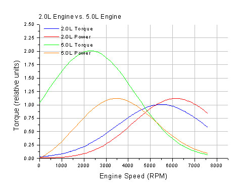
Look a bit further - there are some major differences here:

By the time the 5.0L engine hits 2000 RPM, it’s flying compared to 2.0L engine and at 3000 RPM, you’re almost at the power peak! Weehaa!
If you want to race a 5.0L car with your 2.0L car from stop – you better drop the clutch from no less than 4000 RPM (as we will do in the next section). And don’t shift until red line at 7600.
Which car wins? Don’t know without knowing what the gear ratios on the cars are.

Regardless of gearing however, I think its clear that merely quoting the peak horsepower is useless and is more of an advertising gimmick rather than a useful characteristic.

What Gives You The Rush

Every car enthusiast knows the great feeling that comes when the seats suddenly become pushy, you feel a bit of an adrenaline rush as you catapult from rest up to speed. What’s more, after adding that last modification that promises power gains, one drives around hammering the car searching for confirmation, for that “seat of the pants” feeling that the push in your back is harder than it was before. But exactly what do we really feel? How is our feeling related to the power of the engine, and to the layout of the drive train?

The push that you feel is actually the force applied by the seat upon you to accelerate you from the present speed to the new speed of the car. After all, everything in the car moves down the road at the same speed including you. Our old buddy Newton will tell us that force is a product of your mass and acceleration.

F = m * a    Where F is force, m is mass, a is acceleration.

So assuming your mass stays constant (unless the new modification adds so much power that you end up loosing it at the most important moment ;-), the push that you feel is basically acceleration.

So by describing the acceleration of the car, we can describe what you feel. Alternatively we can simply plot speed of the car vs. time and acceleration would then be the slope of the graph. This method is easy to comprehend and intuitive since our concept of acceleration is that of changing speed.

In the car it is the engine that provides acceleration by developing power and doing  work on the car (see previous discussion). Let us, for right now, ignore the air resistance and power dissapating effects such as friction in the tires, bearings, etc… We can always add them later.  Let’s discuss how this push varies as you go through the entire operating range of the engine in a single gear.

Consider the simplest case – engine develops constant power P anywhere in it’s speed range. This effectively eliminates the element of gearing and gear-shifting. This is not very far from reality as this would be the case with continuously variable transmissions which are able to keep the engine at constant speed regardless of vehicle speed.

Alternatively, we can say that our gears in a regular tranny are spaced such that the engine always operates near the top of it’s power band – a region where power varies little with engine speed. After all, this is the wholly grail of performance power train optimization – tuning the power band and gear spacing such that we can extract the maximum power out of the engine regardless of car’s velocity, if need be.

Those who do not wish to dive into a simple discussion of mathematics that relate physical quantities in this situation can skip this section to the results.

If work = W, power = P, force = F, mass = m, acceleration = a, displacement = x, and time = t,
we can write:

dW = P * dt

dW = F * dx

d here is the total differential of the quantity and it is assumed that force F is in the direction parallel to the direction of car’s movement (basically that you’re not sliding sideways while you’re accelerating).

Then:

F * dx = P * dt

Rearrange to get:

F = P * (dt / dx).

Here dx / dt is the definition of velocity v. So that our expression becomes:

F = P / v.

We know from Newton that:

F = m * a

Substituing in our new definition for F:

a = P / (v * m).

So what do we learn from this simple analysis?

1. It takes more power to provide the same acceleration as at higher speeds than at lower speeds.

2. Weight is definitely not a good thing if you want to “feel the rush”.

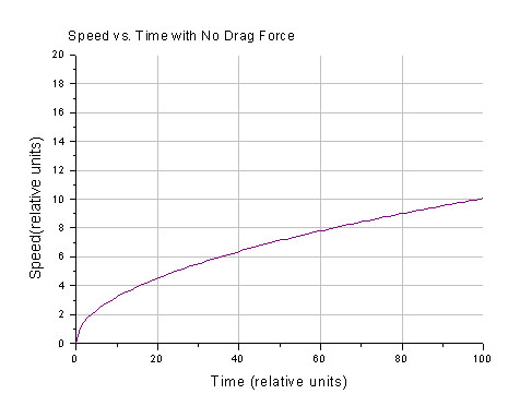
Carrying the math a bit furthe one will see that velocity varies as square root of time:
v = C * Sqrt(t)  where C is a constant which has the mass and power in it as well as some integrating and initial value constants.

The plot of square root function is given below and one can see that even in the ideal case (no air resistance or other frictional drag) the speed increase with time becomes less and less. Thus acceleration keep decreasing from it's initial maximum value.

What is also important that that our constant C carries the power P also under the square root sign. So, for example, increasing the power by a factor of two, only increases the value of the constant by about 1.4 times. The next plot shows the v vs. t graphs from cars with same weight, but with engines developing power 1,2,4,and 9 in relative units (can be HP, can be Watts…).

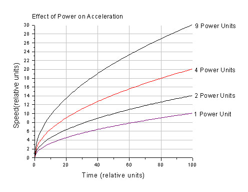
As you can see, increasing power by 9 times (say 900HP vs. 100HP) doesn’t yield 9 times more speed. And we all know what, in real life, the difference between older Ford Escort engine and a highly modified racing Dodge Viper engine is!

Let us now include the air resistance and other parasitic drag.

We will first model it by a simple, yet useful formula:

D = A * v

where D is drag force, A is a constant that lumps together drag parameter specific to the car and environment in which the car moves, and v is, as usual, the speed of the vehicle. This constant A is usually computed experimentally under controlled conditions, but we will use it to show dependencies on parameters.

So let us first balance the forces on the car. Clearly in our model world, we now have 2 forces. The first is the engine force which pushes the car forward (F) and the second is the opposing force of air drag (D).

Balance the forces using first law of Newton:

m * a = F – D = (P / v) – (A * v)

What do we see??
Clearly we see that the value of F falls with rise in velocity and value D grows with velocity. Observe that at small values of v, F > D and (F – D) > 0 . But since they carry opposite signs, F – D will reach zero at some value of v. That value of v is the terminal velocity of the vehicle vt. Acceleration is equal to zero at that point and the car will not accelerate any further.

Let us explore how velocity and acceleration varies with time in this case. Remember that our power and mass of the vehicle are constant regardless of vehicle speed.

After a bit of simple calculus we get:

v*v =  (P/A) – (1/A) * Exp(- X * t)

Here Exp() is an irrational number e ~ 2.7 raised to the power of the argument and X is ( 2* A / m).

The function is plotted below for all values of constants equal to 1.

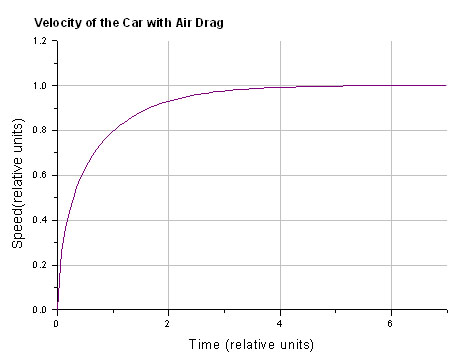
Clearly, as we predicted from force analysis, the Exp(- x * t) goes to zero as time becomes large and we’re left with v = (P/A)^0.5. Thus, in our model system, square root of power developed is directly proportional to the top speed. This is a similar result to the case with no drag except that now we have a terminal top speed. In the case with no drag, the car will accelerate indefinitely.

We continue building up complexity in our model and this time we model our drag force similar to how it is modeled in real world:

D = A’ * v * v

Notice that this a BIG change in the behavior of the drag force. Plot below shows how much faster this new drag force grows with vehicle speed compared to the old, linear one!

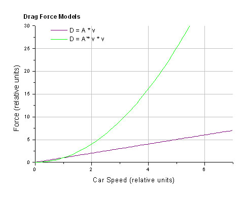
And this, quadratic relationship in speed, is more realistic and is widely used in modeling of drag forces. Notice that A’ is not the same physical quantity as A. Their physical units are different!

So, balance the forces:

m * a = F – D = (P / v) – (A’ * v * v)

Although this new force balance equation seems hardly more complex than in the linear drag case, the expression for velocity as a function of time is very complex! It is not even worth writing it down since we would not be able to make any sense of it by simple analysis.

The plot below shows the typical velocity profile as a function of time.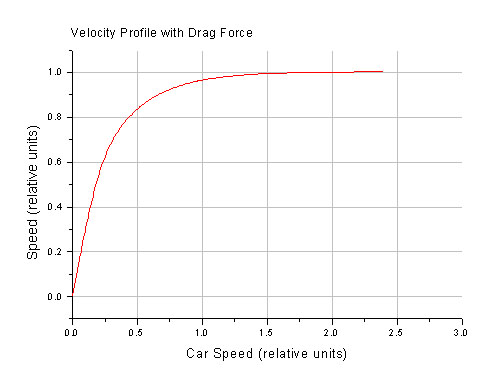 
Again, there is a top speed. In this case, it is not related to power in a simple way.  It is much more useful to look at top speed vs. power plot. This is a good illustration how strongly the top speed depends on power.

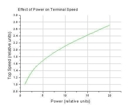
What does it take to double the power of the G2 Legend Type I… that is 400HP? I hear the sound the two turbos… don’t you? Never been done on a street legal Legend car to my knowledge. Yet your top speed only grows 1.3 times! You go from 140 MPH to 182 MPH. Let’s have a milder example – we step up to CAI, Exhaust, chip to gain around 30 HP at the wheels with any luck… what does that mean it terms of top speed increase over stock 140 MPH? Running through the math, you get 145 MPH! Don’t get much for over $1000 spent. Fighting air drag at high speeds is expensive! Our definition of "high speed" depends on the engine and the aerodynamics of the car, of course. "High speed" is where the force of drag is comparable in magnitude to the force that the engine can push the car with. For a Ford Festiva 100 MPH is high considered "high speed". On the other hand, for a 911 Turbo the "high speed" is closer to 150-160 MPH.

While much more complex models exist for modeling drag on the car, they only add details to the last model we discussed. So we will stop here in terms of complexity.
 

Real Power

Let us now, for the sake of wasting some more time, relax the assumption that power is constant and, instead, consider an engine with a power curve as discussed in the previous section about engine tuning. We’re now in a position where we have enough understanding to compute velocity as a function of time for a car that sports an engine that we developed. We will compute the velocity profile as the car accelerates in a single gear from stop.

In order to do this, we must pick a gear ratio to relate the speed of the engine to the speed of the car. To make it simple, we will pick ratio of 1. Why? Because we do not strive to achieve accurate absolute data, but rather we want to compare and as long as we stick with a single ratio, we’re fine. However, with the ratio of 1, our power graph relates power not only to the engine speed, but now to the car’s speed as well!

Additionally, we will assume that the car speed range that we’re working on, is low enough such that drag force is not important. So we will stick with our simplest force balance model:

a = P / (v * m)

Notice that power P is not a constant anymore, but a function of speed!

It is not important how the actual computation is carried out since it is trivial and can be looked up in any numerical methods book.

So, why don’t we compute the speed vs. time profiles for the two cams discussed in the previous section. Just to refresh your memory, below is a power and torque profiles of the two cams.

One has the torque peaking at 5500 RPM and the other at 3000 RPM. The graph below summarises the results.
 

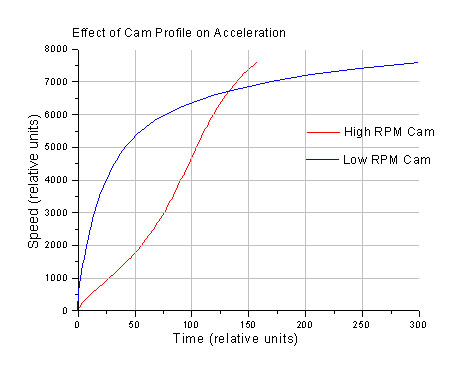
We see, perhaps the most striking proof, that power band position and gearing is what is important. Notice the low RPM cam is faster almost everywhere in the allowed car and engine speed range. The high RPM cam overtakes over only after about 6600 RPM! But, boy, does it take off. The high RPM cam beats its opponent upto 7600 units of car speed by almost a factor 2 in terms of time!

Is this a fair race? Depends up to which speed you’re racing.

Let us launch our cars by dropping the clutch at such engine speed, that each engine starts in the thick of it’s power band. If one examines the two power bands, he/she/it might get the following starting points:

Low RPM Cam Engine: 2000 RPM
High RPM Cam Engine: 4000 RPM

The following graph shows resulting car speed vs. time profiles:

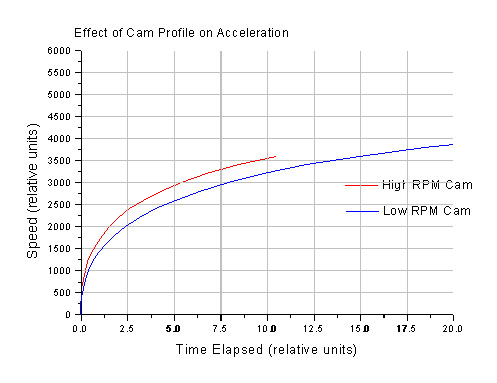
Clearly, the car with more power wins if one fully utilizes gearing and launch to take advantage of high RPM power. Notice that cars make identical peak torque, but exibit vastly different acceleration dynamics because of totally different power bands.
 

The Final Domestic vs. Import Showdown

Let's consider the old “no replacement for displacement and torque” of domestic and import car enthusiasts. Domestic advocates argue that large engines and big torque is the key while the import people quickly throw in the fact that it is the high engine speed power and high power per liter ratio is what counts. Let us see who, if any of them, is/are right.

We look back to our comparison of 5.0L engine with high toque curve, but peak power equal to that of smaller 2.0L engine. Let us compute the velocity vs. time profiles for these two assuming we use proper launch technique for each engine like in the previous example.

We start:
2.0L engine at 4500 RPM
5.0L engine at 2000 RPM

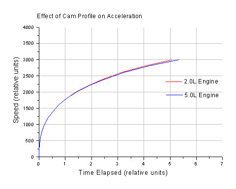
Clearly the simulation data supports our claim that HP is the important factor in car acceleration. Even though 5.0L engine outdoes 2.0L engine in the torque dept. 2 to 1, their acceleration times remain practically identical upto the point where one of the engines runs out its allowed speed range. Furthermore it clearly illustrates that other factors beside the displacement are important.
The above assumes that the two cars weigh the same. It is clear, from our analysis, that if one car is heavier than other, the heavier will loose the speed contest in this case.
 

If you thought this was intense, just wait until we start computing speed with air drag involved! This, in most cases, will not change who finishes first, but would rather separate the looser and winner even more in terms of time required to reach certain speed. Such model would be applicable to high speed, where the drag force becomes comparable in size to the force provided by the engine.

So after this little demonstration, I hope you now will be a bit more about engine design, car kinematics, as well as clever tricky marketing.